---

Visualization Lab

---

1. Molecular Orbitals

Understanding Organic Reactivity

What are some of the fundamental principles that govern the reactivity of molecules? What makes a molecule a good nucleophile or a strong electrophile? How can we predict which position of an aromatic ring undergoes electrophilic or nucleophilic substitutions? The simple understanding that a nucleophile is an electron-rich molecule that attacks sites with low electron density, and that electrophiles are electron-poor molecules that will attack a position of large electron density allows an understanding of many organic reactions.

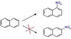
In other situations, this simple understanding is insufficient. For example, how can we rationalize the observed preference for nitration of the 1-position in naphthalene by nitric acid if the total π electron densities in the 1 and 2 position are expected to be the same? In principle, the answer can be reached by considering the structures and energies of the two transition states leading to the two products, but this approach is often impractical.

Frontier Orbital Theory

A powerful practical model for describing chemical reactivity is the frontier molecular orbital (FMO) theory, developed by Kenichi Fukui in the 1950's. An important aspect of the FMO theory is the focus on the highest occupied and lowest unoccupied molecular orbitals (HOMO and LUMO). For example, instead of thinking about the total electron density in a nucleophile, we should think about the localization of HOMO orbital. 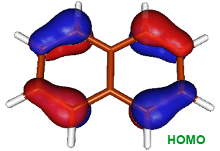Electrons from this orbital are the most available to participate in a reaction. The image on the right shows the HOMO of naphthalene; we can see that the frontier electron density is highest at position 1.

Similarly, the FMO theory predicts that a site where the lowest occupied orbital is localized, is a good electrophilic site. The FMO theory was initially used for explaining the electrophilic substitution in naphthalene but it became gradually clear that the scope of this theory is much broader. For example, the concept of frontier orbital symmetries was successfully used to rationalize the outcomes of cycloaddition reactions and other pericyclic reactions. 

Calculating and Visualizing Molecular Orbitals

Standard quantum chemistry calculations yield delocalized molecular orbital. In Gaussian, the keyword Pop requests printout of molecular orbitals. Alternatively, keywords GFINPUT, IOP(6/7)=3 can be used to greate output that can be visualized with JMOL and MOLDEN. You can download the Gaussian-03 input file and output file that contains a geometry optimzed structure and MO information for naphthalene. You do not need to repeat this calculation because it will be time consuming. Also notice that this calculation included some tretament of electron correlation by invoking the MP2 keyword; the result of this is that many MO orbitals will have fractional populations. You should inspect the input file to make sure that you understand the use of all the keywords.

· Download the latest version of JMOL.

· Open the output file (napthalene_mp2.log) with JMOL. The executable file for JMOL is "jmol.jar."

· The Gaussian output file contains all the intermediate structures from the geometry optimization.  These are all available in JMOL for display.  To select the lowest enegy (optimized) structure click on the JMOL icon in the lower right side of the JMOL window. Select MAIN MENU option, then MODEL 1/8 option (the current structure displayed is the Gaussian input structure), and finally choose the final structure in the list - this is the optimized geometry.

· You are now ready to display the MOs as isocontour surfaces around the molecule. There are two ways to do this:

1.In the MAIN MENU (from JMOL icon) select SURFACES, then MOLECULAR ORBITALS. You will then see another window with numbers (in groups of 25) on it. These are the molecular orbitals, the are numbered from the lowest energy orbital to the highest (the energies of these orbitals in Hartrees are also listed). Select the first orbital. You should see MOs centered at atoms: these are the core orbitals at heavy atoms that are not involved in bonding. Inspect some other

2.In the FILE pulldown menu select SCRIPT. The JMOL Script Console will open.  This provides a very powerful way to interact with JMOL. In the script console window type the command mo 1 and hit return. You should see the first molecular orbital appear.  You can change the look by typing mo fill nomesh followed by return.  This should make the mo look solid rather than a mesh.  Now type mo translucent followed by return.  What happens now? There are many things you can do.  Documentation for this interactive scripting language is available from St. Olaf College. From the documentation menu open the "mo" link for command usage and examples.

· Using either method, select the highest energy occupied MO (the least negative energy). This is one of the bonding Pi orbitals.

· Compare your result with the image in the tutorial.

· Play around some more.

Molecular Orbitals in Conjugated Systems

According to the frontier orbital theory, the chemistry of conjugated π systems is largely determined by the HOMO and LUMO π orbitals in the reactant molecules. The outcome of reactions involving interaction of π orbitals can be rationalized using the concepts of orbital phase and symmetry. The figure on the right illustrates what is meant by the orbital phase using 1,3-butadiene as an example. In this molecule, four atomic p orbitals form four π molecular orbitals. The four molecular orbitals differ by the extent of favorable overlap, and thus in energy. The lowest energy MO forms from the in-phase overlap of all four p atomic orbitals; the next one forms when two pairs or in-phase atomic orbitals overlap; the third when one pair of in-phase atomic orbitals overlaps, and the highest energy molecular orbital forms when there are no in-phase overlaps. The MO's are filled with electrons starting with the lowest-energy orbital such that two electrons occupy an MO. In case of 1,3-butadiene, there are 4 π electrons, thus the second lowest-energy orbital is the HOMO.

The Diels-Alder Reaction

The Diels-Alder reaction is a cycloaddition reaction between a conjugated diene and dienophile.

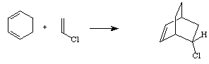
Diels-Alder reaction has high synthetic utility for making unsaturated six-membered rings. The reaction with unsubstituted dienophile (as shown above) is very slow but the Diels-Alder reactions occur readily when the alkene has a electron-withdrawing substituent. For example, acrolein is a good dienophile. Cycloalkenes, especially ones where the double bond is conjugated to a carbonyl, can be used as dienophiles. The diene is required to have an s-cis conformation and cyclic dienes work well in this reaction. For example, a reaction between 1,3-cyclohexadiene and chloroethene yields a bicyclic reaction product.

Note that chlorine is a relatively poor π-electron withdrawing group and the reaction above in not very fast. Interestingly, many Diels-Alder reactions occur much faster in water than in organic solvents. Scientists are still working on finding out why aqueous environment accelerates this reaction.

Molecular Orbitals in Diels-Alder Reaction

The Diels-Alder reaction is highly stereoselectivive: cis-substituted dienophiles yield cis-substituted cyclohexenes and trans-substituted dienophiles yield trans-substituted cyclohexenes. Stereoselectivity in Diels-Alder reaction can be rationalized considering the overlap of HOMO of one reactant with LUMO of the other.

· Using GridChem and Gaussian calculate the MOs for ethylene and 1,3 butadiene.  You can obtain initial structures from Chem3D or any other program to construct molecules that you are comfortable with.  Minimize the geometry with some simple force field (MM2 in Chem3D).

· Use the same keywords from the example napthalene input file.

· Notice that the Gaussian program uses keywords to decide what kind of calculation to perform and what kind of results to produce. The extra keywords, like GFINPUT, IOP(6/7)=3, and 6D or 5D are required by MOLDEN or JMOL, respectively, to visualize results from Gaussian.

· Use JMOL and WORD (or EXCEL) to construct a table showing π molecular orbitals for ethylene (dienophile) and 1,3-butadiene. In particular, you will be interested in the HOMO and LUMO for each (you may also want to look at HOMO-1, LUMO+1, and LUMO +2 if you want to see which reactant orbitals become product orbitals).

· Remember that you want to select the  minimized  geometry from the output file for JMOL to display.

· Use your computed MOs to verify the reaction mechanism above.  Almost any organic text can be used for additional information.

You can read more about the frontier orbital theory from Kenichi Fukui Nobel Prize lecture.

2. Molecular Surfaces

Molecular Shape Surfaces

The shape of a molecule is determined by the electron density of the molecule and this electron density depends on the atomic composition of the molecule. One way to determine molecular shape is to calculate electron density and display the region where electron density is larger than some cut-off value as a three-dimensional surface. Such calculations necessitate quantum chemical approach and are possible with not too large molecules. For larger molecules, Connolly surfaces and solvent-accessible surfaces can be calculated rapidly based on empirical van der Waals radii of atoms.

Electrostatic Potential Surfaces

Electrostatic potential surfaces are valuable in computer-aided drug design because they help in optimization of electrostatic interactions between the protein and the ligand. These surfaces can be used to compare different inhibitors with substrates or transition states of the reaction. Electrostatic potential surfaces can be either displayed as isocontour surfaces or mapped onto the molecular electron density. The latter are more widely used because they retain the sense of underlying chemical structure better than isocontour plots.

Example: Oxamic Acid

This tutorial illustrates how to use quantum chemistry calculations to generate and display molecular electron density surfaces and map electrostatic potential values to the surface. You will compare two conformers of oxamic acid. Oxamate, anion of oxamic acid is a powerful inhibitor for Plasmodium falciparum lactate dehydrogenase and thus may serve as a fragment or lead in developing novel anti-malaria drugs. The molecule has two low energy conformers that differ in the dihedral angle about the central C-C bond. These conformers are shown in the image on the right.

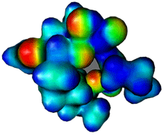
Your task is to calculate and display electrostatic potential of cis and trans oxamic acid. Molecular surfaces should be calculated based on optimized molecular geometries. While molecular mechanics force fields can be used to generate reasonable initial geometries, it is considered a good practice to optimize molecular geometries with quantum mechanical methods prior to generation of electron molecular electrostatic potential surfaces. In this tutorial you use Chem3D to construct and minimize the cis and trans oxamic acid structures using the MM2 Force Field.  The quantum chemistry program Gaussian was used to perform geometry optimization for the two conformers. You will use GRIDCHEM to launch quantum mechanical geometry optimizations but keep in mind that optimizing a larger molecule using accurate QM methods can be very time-consuming. The calculation will be performed at the Moller-Plesset second order perturbation theory level with a moderate-sized basis set to describe molecular orbitals. Specifically, a 6-311+G(d,p) basis set will be used which allows for some polarization of electron density on both heavy atoms and hydrogens. In computational jargon, the molecule will be optimized at the MP2/6-311+G** level. The comparison of relative energies of the two conformers suggests that s-trans conformer is more stable by 1.68 kcal/mol.

· JMOL Properties Visualization from Gaussian-03 Output File

1.Notice that the Gaussian program uses keywords to decide what kind of calculation to perform and what kind of results to produce. The extra keywords, like GFINPUT, IOP(6/7)=3, and 6D or 5D are required by MOLDEN or JMOL, respectively, to visualize results from Gaussian. You can modify the Keyword lines to add advanced options. For example, to request a rather expensive CCSD/cc-pVTZ calculation, you could change HF/6-31G** to CCSD/cc-pVTZ. Gaussian options are discussed in detail at http://www.gaussian.com/g_ur/keywords.htm

2.Give an unique and easy-to-identify name to the job. For example, you may name the trans conforner oxamic_trans.

3.The title line is for optional comments. People typically add some description as of the purpose of this calculation. 

4.You can cut and paste the the xyz-coordinates from Chem3D.

5.Detrmine the difference in energy between the two conformers.

6.Display the MOs, especially the HOMO and LUMO, for these conformers using the methods outlined above.

7.Now let's map the the molecular electrostatic potential (MEP) onto the solvent_accessible surfaces for each conformer. Ideally, one would map the  MEP onto the molecular electronic density, however, one needs to calculate a CUBE file from the Gaussian checkpoint file to complete this task (see below). Open the JMOL Srcipt console and type: isosurface delete resolution 6 solvent map mep. Describe what see.  What is the significance ?

8.Play around with some of the surfaces.  Check out this Isosurfaces Examples page for some ideas..

· JMOL Properties Visualization from Gaussian-03 CUBE File.  The CUBE file are very large, even compressed.  These may take a while to download.

1.Download CUBE files for trans-oxamic and cis-oxamic acids (you do not need to unzip these files, JMOL can read the zipped files):

§ trans_den.cube.gz & cis_den.cube.gz  -  These files contain the electron density data.

§ trans_pot.cube.gz & cis_pot.cube.gz  -  These files contain the electrostatic potential data calculated from the electron density and nuclear conformation.

§ trans_homo.cube.gz & cis_homo.cube.gz  -  These files contain the volumetric data for the HOMO.

§ trans_lumo.cube.gz & cis_lumo.cube.gz  -  These files contain the volumetric data for the LUMO.

2. Open JMOL and the JMOL Srcipt console.

3.Now you must set the PATH to your working directory in the JMOL Srcipt console.  Type: set defaultdirectory "path-to-working-directory" The quote marks must be used for your directory.

4.Let's start with the trans-oxamic acid.  Load the coordinates from the density file.  Type: load trans_den.cube.gz   - you should see the molecule in the JMOL dispaly window. You can make it a stick model by using the pulldown menu DISPLAY:ATOM:NONE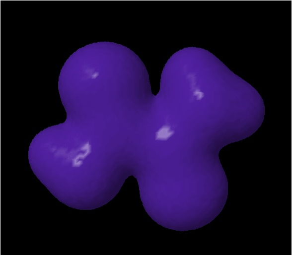

5.Now display the electron density by typing  isosurface "trans_den.cube.gz"  You should see something like the image to the right.   

6.You can change the value of the isosurface by using the cutoff option:   isosurface cutoff 0.01 "trans_den.cube.gz"   This just changes the value of the electron density used to establish the surface.

7.You can also change the color of the surface; for example:   color isosurface red

8.You can also  make it translucent:   isosurface translucent  or a mesh:   isosurface nofill mesh

9.The command isosurface delete will delete the surface.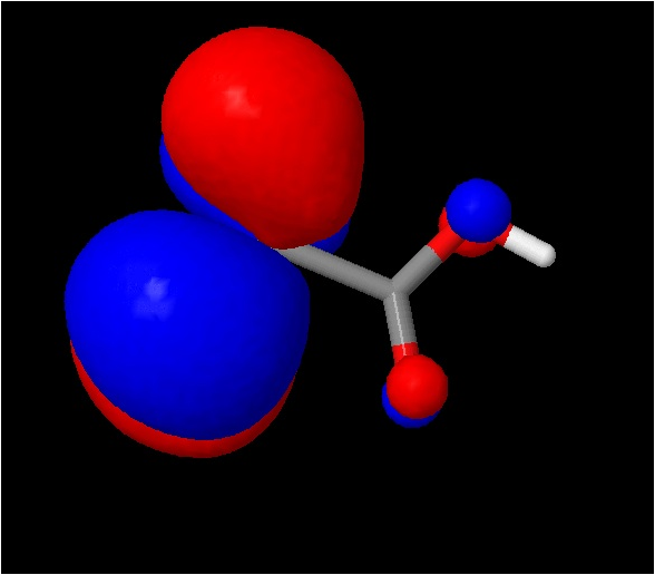

10. Now we will plot a molecular orbital (the sign option tells Jmol to plot both the positive and negative lobes):    isosurface sign "trans_homo.cube.gz"

11. 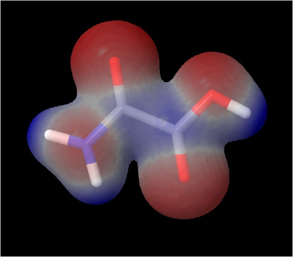You can also map the electrostatic potential onto the elctron density isosurface, similary to step 7, above.  "isosurface trans_den.cube.gz" colorscheme "rwb" color absolute -0.1 0.3 map "trans_pot.cube.gz"     Try not changing the color scheme ("isosurface trans_den.cube.gz" map "trans_pot.cube.gz") and see what happens.

12. You can also plot planes through volumetric data rather than plot isosurfaces.  Pick three atom to form a plane (C2 C3 & N4).  Then use these three command lines in sequence:

§ draw myplane (C2) (C3) (N4)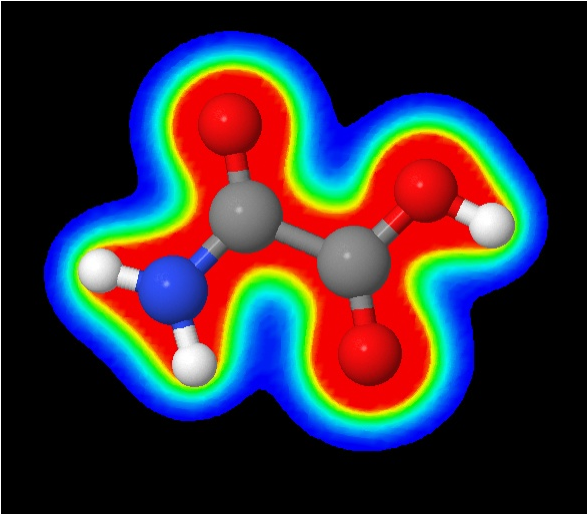

§ draw off

§ isosurface plane $myplane  colorscheme "roygb"  color absolute 0.01 0.15 reversecol "trans_den.cube.gz"

13. Repeat for the cis-oxamic acid and note differences.  Play with this - it is very powerful and instructive.